Advanced forecasting calculations complement the current forecasting to help you delve more deeply into how your products should be managed for replenishment. The system looks through the sales history going back a specified amount of time. Eclipse uses your selected group and goes back 52 weeks to gather the most recent sales history on your buy line or product set. Then, using that information applies your selected advanced forecast method. The system records the values by product for each of these methods with the product's file. Demand Calculation Audit updates with the current method.
Note: You can add advanced forecasting method results to a user-defined queue using the BR_BEST_FIT and BR_ADV_FRCST dictionaries. For more information about user-defined views and user-defined queues, see Creating User-Defined Views and Creating User-Defined Queues.
See Assigning Advanced Demand Forecast Methods to indicate which method you want to use.
In forecasting inventory, smoothing refers to finding the demand by removing the random variations that may occur in the purchasing history. This helps determine demand patterns more accurately, so that you do not purchase for those exceptional sales or exceptional periods in the life of the warehouse. For more information about smoothing factors, see How Advanced Demand Forecasting Works .
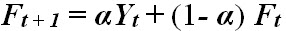
The simplest form of exponential smoothing is given by the following formula:
Where α is the smoothing factor and 0 < α < 1. This means that the smoothing is a weighted average of the previous data and the previous smoothed statistic. For Eclipse, this means the system uses the previously calculated smoothing factor and the previously calculated demand within the specified time frame and uses the average to determine the demand. Exponential refers to the fact that you use the smoothing factor back into itself on each subsequent demand calculation. Therefore, it changes exponentially.
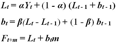
The Holt method calculates the same way as the single exponential smoothing, but calculates using the trending factor in addition to the smoothing factor. The formula calculations are as follows:
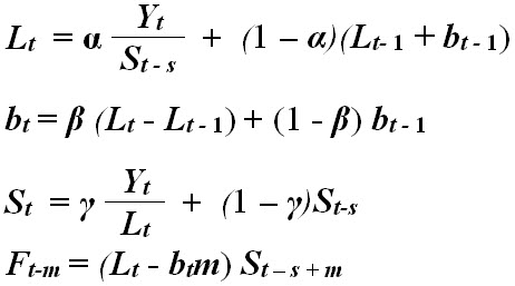
The Holt-Winters method calculates the same way as the standard Holt method, but uses seasonality in addition to the since exponential smoothing and trending factors. To initialize the Holt-Winters calculations, the system uses back-casting. This allows the system to handle a wider variety of sales patterns without producing inaccurate forecasts.
The year is broken into 52 buckets, or 52 weeks' worth of data. For Holt-Winters, each bucket is adjusted according to its seasonal score. This means the system provides a "at this time of year, the sales are x% of normal." The seasons score for that bucket is updated according to the gamma value.
For items that pass the seasonality test, the system runs the Holt-Winters method.
Note: Holt-Winters calculations are not made with less than three years demand history.
For both Single Exponential Smoothing and Holt methods, the system uses a weekly demand divided by seven multiplied by 30 to get the monthly demand value:
monthly demand = (weekly demand / 7) x 30
For Holt Winters method, because the forecast is more than a single week, Eclipse uses four 2/7ths of a week and make that the monthly demand. Eclipse divides that value by 30 to find the daily demand.
Runs as if the product is set to standard method for each method (above) individually and without relying on information from the other calculations. For more about how the system creates and manages best fit calculations, see How Eclipse Calculates Best Fit.